Alternative models to portfolio selection in the Brazilian market.

Helder Parra Palaro

Bayes Capital Management

Abstract

We examined alternative risk-factor models for portfolio construction in the Brazilian equity market. We considered 8 linear models and 4 non-linear models, and also a mixture of 4 models. For long-only (LO) and long-biased (LB) portfolios, the IPCA (instrumented principal component analysis) and the mixture of models slightly outperform the traditional method of portfolio construction on a risk-adjusted basis. For long-short (LS) portfolios, the traditional method is still superior.

1. Introduction

The main interest of the asset pricing area is to explain why different assets produce different returns.

The CAPM model was introduced independently by Sharpe (1964), Linter (1965) and Mossin (1966). Using the Markowitz framework (1952), the model assumes that just one risk factor is enough to capture the difference in asset expected returns: the market risk, which is the only systematic risk, therefore non-diversifiable. Different assets have different exposure to the market risk. This exposure is captured by the beta coefficient of each asset, which measures the covariance between the returns of each of these assets and the market risk.

Ross (1976) relaxed the CAPM concept, assuming that the asset expected returns depend not on only one, but several risk factors. In this case, the risk factors can be relevant macroeconomic variables or company characteristics.

Fama and French (1993) formulated a three risk factor model: market risk, value (measured by the ratio between book value and market value) and company size. Carhart (1997) added a fourth risk factor, known as momentum, which depends on how much the asset price went up or down in the last year. These methods sort the assets by risk factors, and then create long/short portfolios.

The quest for risk factors generated a situation described by Cochrane (2011) as “factor zoo”, where hundreds of company characteristics were identified as possible influence on asset returns. However, many of these characteristics are possibly proxy for the same risk factors, and hence redundant.

Kelly et al. (2019) propose the IPCA (instrumented principal component analysis) model for asset pricing. As in traditional approaches, expected returns of assets are written as compensation for non-diversifiable risk factors. However these risk factors are not specified a priori, but assumed as latent, and estimated by principal component analysis. Company characteristics are used as instrumental variables on the estimation of asset betas, which are a map between risk factors and expected returns.

Recently, machine learning models started to be used in the asset pricing area. These models allow the treatment of linear and non-linear association in high dimension data, and use regularization methods to avoid overfitting.

Gu et al. (2020) examine several of these methods for about 30,000 individual stocks in the US. The predictors are 94 company characteristics, as well as 74 sector dummy variables, and 8 time series. The results obtained by the authors show that linear models have good performance when there is some kind of penalization of dimension reduction. Non-linear model improve the quality of the predictions. “Shallow” learnings works better than “deep learning”, where the model have several layers.

Gu et al. (2021) extend the IPCA model of Kelly et al. (2019) to the non-linear case, using neural networks known as auto-encoders to model the association between risk factors and covariates.

Rubesam (2019) applies an approach similar to Gu et al. (2020) for 572 stocks in the Brazilian market in the 2003-2018 period. He considers 86 company characteristics. Portfolios are formed according to traditional long-short methods and also through an ERC (Equal Risk Contribution) approach. The non-linear models produce disappoint results. The ERC method which combines several machine learning predictions produce the best results.

2. Machine learning

Statistical learning and machine learning emerged from different areas (statistics and computer science), but the difference between them is becoming each day less distinct. Both focus on supervised and unsupervised learning (Hastie et al. (2009)). In supervised learning, which is the approach used in this report, the aim is to use the independent variables X₁, X₂, …, X_p (or inputs) to predict the response variable y (or output). If the variable y is categorical, it is a classification problem. If it is a continuous variable, it is a regression problem. We are going to use both models here. We must then estimate the function f, where y = f(X | β). The function f depends on the parameters β which must be estimated (model training).

The dataset (X_train,y_train) used to train the model is known as training data. After training, we have the prediction function f_opt( | β_opt). We then use a new dataset (X_test,y_test), independent from the training data, called test data. Finally, we can estimate y_test by f_opt(X_test| β_opt).

There are also hyperparameters which control the learning process via the model complexity. A very complex model can cause a situation called overfitting, where there is a good fit to the training data, but not to the test data. On the other hand, a very simple model may not capture all the association between variables.

The simples model considered here is the multiple linear regression. This method assumes that the response variable is a linear function of the independent variables. We have then y = Xβ, and there are not hyperparameters.

The Ridge and LASSO regression methods impose a penalization on the estimation of the coefficients of the linear regression, forcing the coefficients to values more similar between each other. The penalization is quadratic in the Ridge regression case and in absolute values in the LASSO case. These techniques are called regularization. They reduce the model variance in a significant way, introducing some bias. The hyperparameter controls the amount of penalization on the coefficient estimation.

When there are several highly-correlated independent variables, an alternative is to reduce the dimension using principal component analysis. The PCR and PLS methods use this technique. In the PCR case, the first step is to create new variables Z₁, Z₂, …, Z_m which are the linear combinations of X₁, X₂, …, X_p which explain the largest variation of the original data, and are orthogonal between each other. After that, the response variable y is regressed on the variables Z instead of the original variables X. In the PLS case, the linear combinations are built also orthogonal to the response variable y. The hyperparameter for these methods if the number of principal components.

The IPCA model is also a linear method, which reduces the dimensionality of the estimation problem. As specified in the introductory section of this report, this method preserves the interpretability of the individual asset expected returns as a combination of betas (factor loadings) multiplied by risk factors.

We also consider two linear classification methods. The first one is the Logistic Regression, originally modelled by Berkson (1944), which in its simplest form uses a logistic function to model a binary dependent variable. The second is the Linear Discriminant Analysis (LDA), from Fisher (1936). It generates discriminate functions, which are linear combinations of the independent variables. It assumes multivariate normality, which can be more efficient if this assumption holds, but otherwise the logistic regression is more robust.

The first non-linear model considered here is the random forest model. Decision trees (Breiman et al. (1984)) partition the sample space (all possible values of X₁, X₂, …, X_p) into disjoint regions, where the response is considered as the mean of y for each region. This partition is done via an algorithm which determines, on each step, one variable and a split point where the sample space will be divided. The number of partitions determine the tree complexity. Random forests (Breiman (2001)) are based on the construction of a large number of uncorrelated decision trees, and averaging them. It is an application of the statistical technique known as bagging, where the average of several weak predictors (with high variance but no bias) produces a strong predictor. The procedure to build non-correlated tree is to randomly choose a subset m of p independent variables, where m <= p. This avoids that one variable, or a small number of variables, dominate the way most splits will occur. The hyperparameters are the level of tree complexity and the number m of variables to be chosen for each individual tree.

Neural networks are non-linear models formed by one or more intermediate layers (hidden layers) (Bishop (1995) and Ripley (1996)). In the first layer, we create new variables Z₁, Z₂, …, Z_m , defined by Z_i = σ(a₀ + a_i^tX), where σ is called the activation function. An activation function normally used is the sigmoid function, given by σ(x) = 1/(1+exp(-x)). After that, we can have other intermediate layers, where the variables generated on the first layer are combined. Finally, in the last layer, we have the response variables to be predicted. The model estimation uses an algorithm named “backpropagation”. The hyperparameter controls the backpropagation stop to avoid overfitting.

The last machine learning model is a classification model, the Support Vector Machine (SVM) model. The method is well described in Vapnik (1996). The method constructs hyperplanes which maximizes the distance to training data point of any classes. For many data sets, the classes are not linearly separable, so the original data is mapped to higher or infinite dimensional space. Kernel functions can be used to make the method non-linear.

3. Data

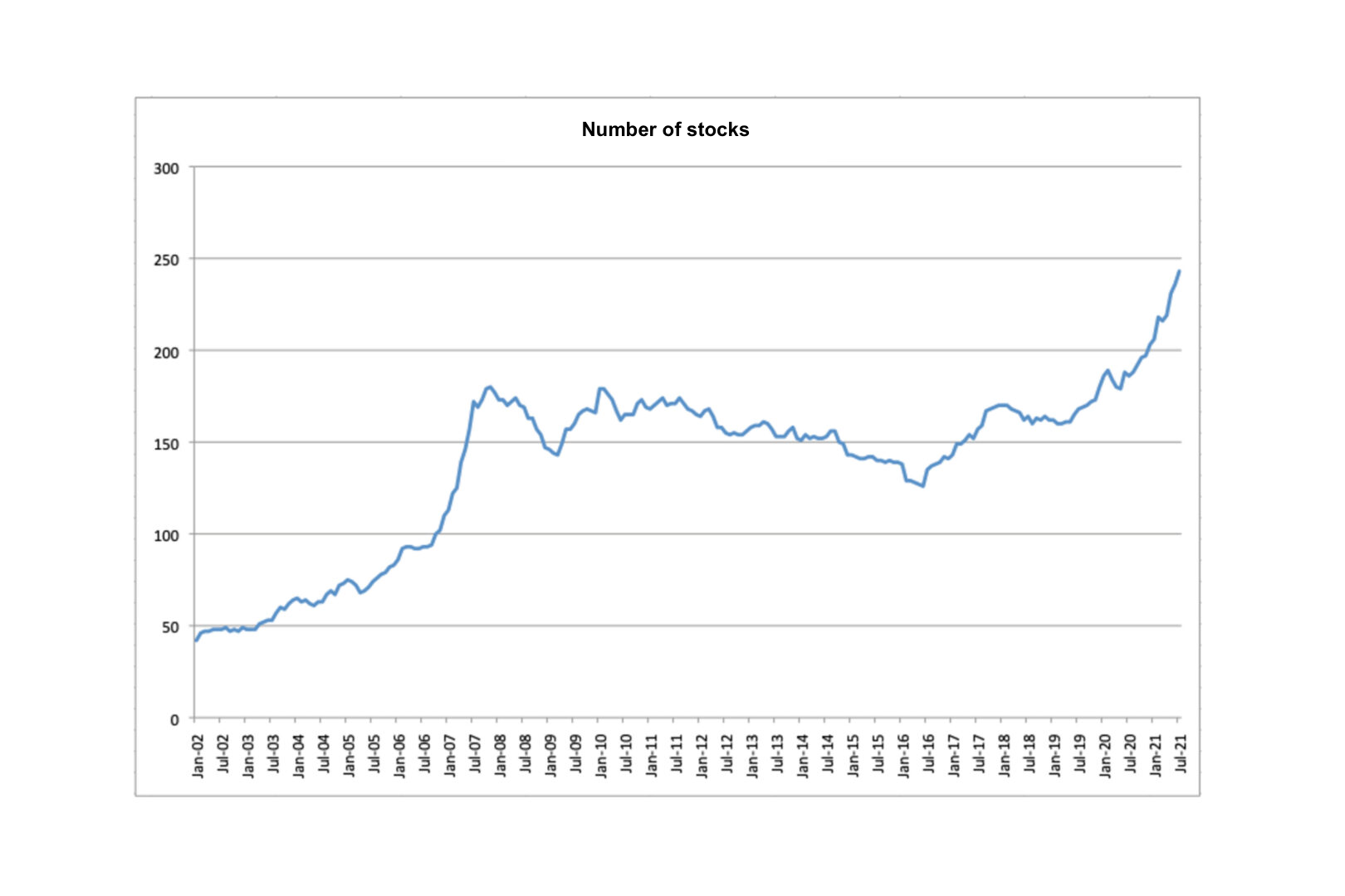
The dataset comprises 413 Brazilian stocks in the January 2003-July 2021 period. We calculate monthly returns for these stocks. In each month, we use only the stocks which pass our liquidity filter requirements. (Figure (2)).

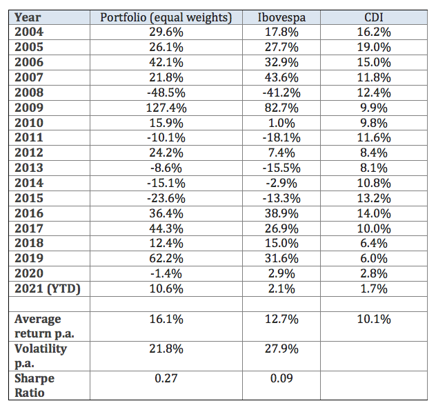
Building an equally-weighted portfolio with the stocks which pass the liquidity filter¹, we obtain the results on Table 1². We can see that our universe of stocks is more diversified and outperforms the Ibovespa index, which is too concentrated in a few specific sectors.

---

1 Average volume above R$ 200.000,00.

2 In all this report we consider typical equity trading costs and monthly rebalance, according to our live funds.

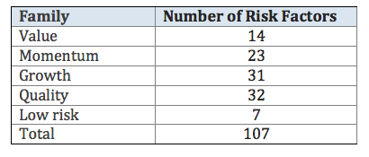
Besides the monthly returns, our database, which is being improved since the first version of our risk-factor model in 2012, comprises 107 fundamental e technical indicators for each company. These indicators are created from balance sheet data and market data, like price, volume, liquidity, etc. As mentioned to the introductory section of this report, these indicators are known as risk factors. They can be grouped in 5 families of risk factors, as described in Table 2.

4. Methodology

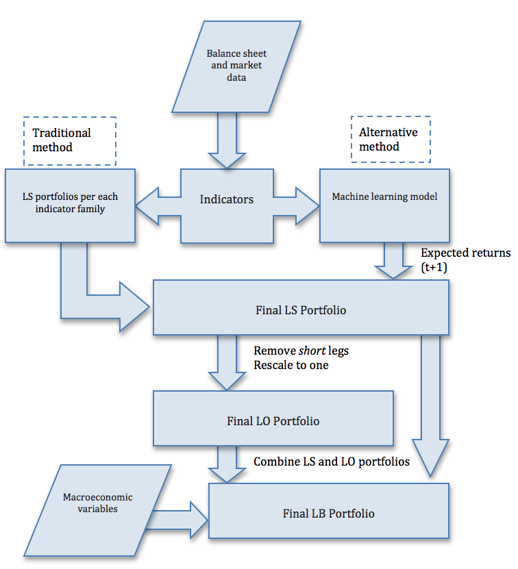
Figure 3 shows a diagram of the portfolio generation method for LS (long-short), LO (long-only) and LB (long-biased) portfolios. In the first step, we generate indicators for all companies in our database. In the traditional method, these indicators are combined using a proprietary process to produce 5 long-short portfolios, one for each family. These 5 portfolios are combined to create a final LS portfolio¹. If we force the negative weights to zero and rescale the portfolio, in order to the weights add up to one, we obtain an LO portfolio. Finally, we use a proprietary system, which is a tactical allocation system which varies the allocation between the portfolios LO and LS, to produce an LB (long-biased) portfolio. This tactical system uses macroeconomics variables, and it is able to vary the gross and net exposure of the portfolio according to the macroeconomic environment.

1 We rebalance monthly.

For the machine learning methods, the indicators are transformed directly into an LS portfolio, skipping the creation of the LS portfolios for each family of indicators. For the regression models, we simply estimate the expected return of all the stocks for the next month, and then create a portfolio with long positions for the 20% largest expected returns, and short positions for the 20% lowest expected returns. For the classification models, we estimate the classes (long/flat/short). After that, we proceed as in the traditional method to create LO and LB portfolios.

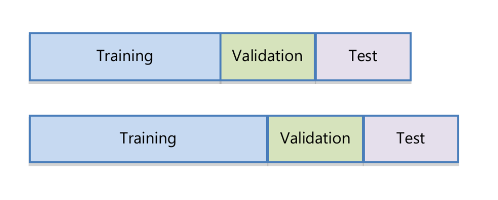
The machine learning models are estimated using an expanding window. As in Rubesam (2019), we consider a 24-month initial window as training data. Following that, we use the next 12 months to estimate the hyperparameters (validation data), and finally we apply the estimated model (including parameters and hyperparameters) for the next 12 months (test data). The training data window is then expanded by 6 months. The process is illustrated in Figure 4.

We use the same data transformation as in Rubesam (2019). The monthly returns and also the indicators are transformed into rankings and standardized to the interval (-1,1). This reduces the influence of outliers, and therefore make the model estimation more robust.

We considered eight linear models: OLS (ordinary least squares), Ridge regression, LASSO, PCR, PLS, IPCA, Logistic Regression and LDA. Additionally, we considered four non-linear models: random forests, two architectures of neural networks and SVM with radial kernel.

We also considered a mixture model, which is the simple average of four models: Ridge, IPCA, random forests and the simplest of the two neural networks. We labelled this model as “Comb4”.

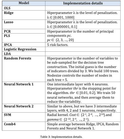
Some implementation details are described in Table 3. All the implementation was in R language, using several packages, such as ‘glmnet’, ‘pls’, ‘caret’, ‘randomForest’, ‘plm’ and ‘neuralnet’. The IPCA model was implemented in Matlab.

5. Results

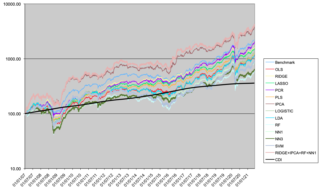
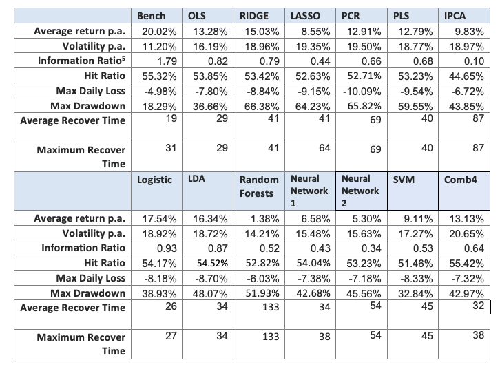
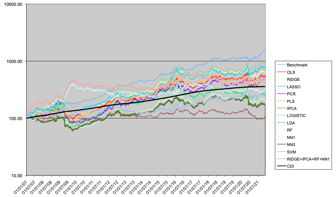
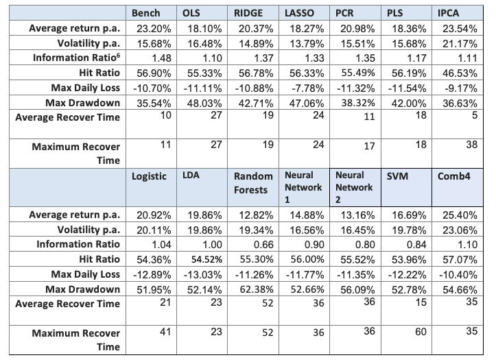
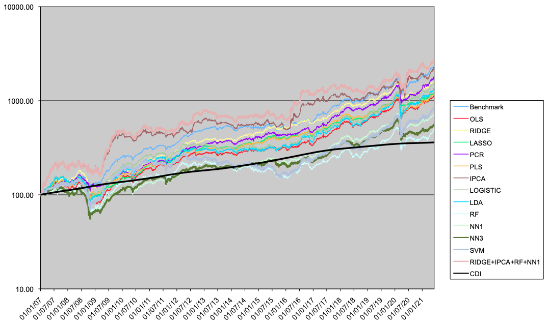
In this section we present the results for the LO portfolios (Table 4 and Figure 5), LS portfolios (Table 5 and Figure 6) and LB portfolios (Table 6 and Figure 7).

In the long only case, the linear model have better results than the non-linear ones. The regularization methods (like Ridge regression or PCR) improve the performance compared to OLS. Two models outperform the benchmark (traditional portfolio formation), the IPCA model, and the Comb4 model. These two models outperform the benchmark both in performance and drawdown measures.

In the long-short case, no alternative model comes close to the benchmark. The only ones with a reasonable performance are the Logistic regression, the LDA and the Ridge regression.

Considering the long-biased case, which is a combination of the LO and LS portfolios according to our tactical allocation macro model, the results of the linear alternative models outperform the non-linear models, but not the benchmark. Ridge, PCR, IPCA and Comb4 produce the best performance, and the Ridge regression is the best in terms of drawdown.

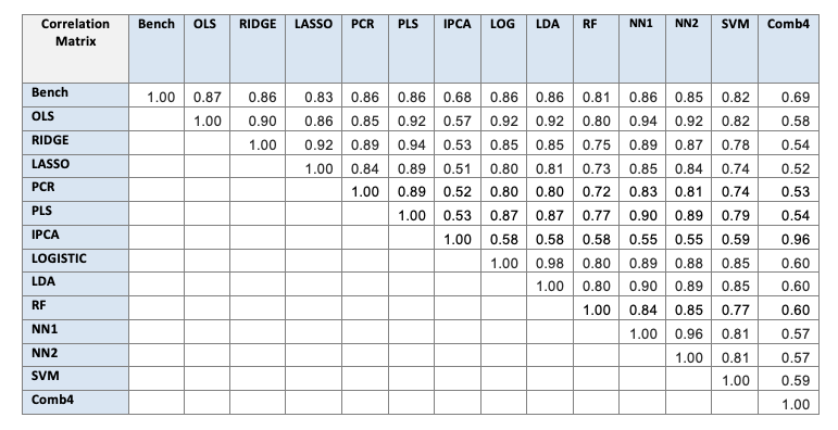
Table 7 shows the correlation between LB portfolios. The linear models have a reasonably high correlation between themselves, except for the IPCA, which works in a completely different way. The correlation between the non-linear models is also high. The models IPCA and Comb4 are the less correlated with the benchmark (traditional portfolio formation).

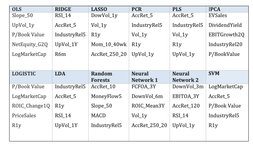
In Table 8 we can see the five most important indicators for each model, obtained out-of-sample. We can see that the technical indicators are the most important for most of models, except the IPCA model, where fundamental indicators are chosen.

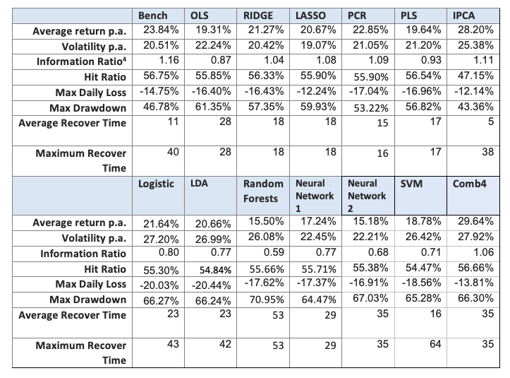
4. We obtain the information index dividing the annualized average return by the annualized volatility. This is a different formula from the Sharpe ratio, where the risk-free return is deducted from the performance.

6. Conclusion

We tested several alternative models for equity portfolio construction in the Brazilian market. We built long-only, long-short and long-biased portfolios. We considered eight linear models, four non-linear models and a combination of four of these models.

The results show that for long-short portfolios, the traditional method of portfolio construction is still the best. For the long-only and long-biased cases, we believe there is a justification for an experimental allocation to the alternative models. The main candidates for this allocation are the IPCA model, the linear models with penalization, or the combination of four models. Given that the IPCA model has the best interpretability and theoretical foundation, we believe it is the best candidate.

7. References

• Berskon, J. (1944), “Application of the logistic function to bio-assay”, Journal of the American Statistical Association, 39, 357-365.
• Bishop, C.M. (1995), “Neural networks for pattern recognition”. Oxford university press.
• Breiman, L., Friedman, J., Olshen, R. and Stone, C. (1984), “Classification and regression trees”, Wadsworth, New York.
• Breiman, L. (2001) “Random forests”, Machine Learning, 45, 5-32.
• Carhart, M. (1997), “On persistence in mutual fund performance”, , 52 (1), 57-82.
• Cochrane, J. (2011), President address: Discount rates.
• Fama, E. F. and French, K. R. (1993), “Common risk factors in the returns on stocks and bonds”, Journal of Financial Economics 33(1), 3–56.
• Fisher, R. A. (1936), “The use of multiple measurements in taxonomic problems”, Annals of Eugenics, 7: 179-188.
• Gu, S., Kelly, B. and Xiu, D. (2020), “Empirical asset pricing via machine learning”, The Review of Financial Studies 33 (5), 2223-2273.
• Gu, S., Kelly, B. and Xiu, D. (2021), “Autoenconder asset pricing models”, Journal of Econometrics 33 (5), 2223-2273.
• Hastie, T., Tibshirani, R. and Friedman, J.H. (2009), “The elements of statistical learning: data mining, inference, prediction”, Second Edition, Springer Verlag, 2009.
• Kelly, B., Pruitt, S. and Su, Y., (2019), “Characteristics are covariance: a unified model of risk and return”, Journal of Financial Economics, 134 (3), 501-524.
• Lintner, J. (1965), “The valuation of risk assets and the selection of risky investments in stock portfolios and capital budgets”, Review of Economics and Statistics, 47, 13-37.
• Markowitz, H. M. (1952), “Portfolio selection”, Journal of Finance, 7, 77-91.
• Mossin, J. (1966), “Equilibrium in a capital asset market”, Econometrica, 34, 768-783.
• Ripley, B. D. (1996), “Pattern recognition and neural networks”. Cambridge University press.
• Ross, S. (1976), “The arbitrage theory of capital asset pricing”, Journal of Economic Theory, 13 (3), 341-360.
• Rubesam, A. (2019), “Machine learning portfolios with equal risk contributions”, Working paper, IÉSEG school of management.
• Sharpe, W. (1964), “Capital Asset Prices: A Theory Of Market Equilibrium Under Conditions Of Risk,” Journal of Finance, 19 (3), 425-442.
• Vapnik, V. (1996), “Statistical Learning Theory”, Wiley, New York.